Evaluator

This example shows how to use the Evaluator class to evaluate the errors for the given configurations with the trained potential.

import logging

import ase.io
import matplotlib.pyplot as plt

from motep.evaluate import Evaluator
from motep.io.mlip.cfg import write_cfg
from motep.io.mlip.mtp import read_mtp

If you need a log, you can set the following.

logging.basicConfig(level=logging.INFO, format="%(message)s")

We first load the trained potential.

mtp_data = read_mtp("final.mtp")
mtp_data.species = [6, 1]

We then load/make the configurations to evaluate. In this example, we just evaluate the training dataset itself.

images_training = ase.io.read("../0.0_train/ase.xyz", index=":")
images_in = images_training

We then make the Evaluator class and grade the images by the potential.

evaluator = Evaluator(mtp_data)
images_out = evaluator.evaluate(images_in)

The energies and the forces with the given potential are stored in atoms.calc.results. We can access them by, e.g., atoms.get_potential_energy().

images_out[0].get_potential_energy()

np.float64(-199.61934293654744)

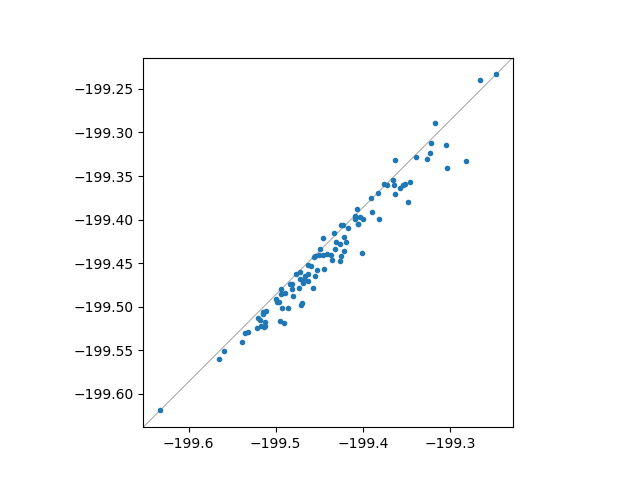
We make a parity plot to compare the original and the evaluated energies.

targets = [atoms.calc.targets["energy"] for atoms in images_out]
results = [atoms.calc.results["energy"] for atoms in images_out]
fig, ax = plt.subplots()
ax.plot(targets, results, ".")
ax.axis("equal")
ax.set_box_aspect(1.0)
ax.axline(
    (0.0, 0.0),
    (1.0, 1.0),
    color="#b0b0b0",
    lw=0.8,
    zorder=0.0,
    transform=ax.transAxes,
)
plt.show()

We finally store the evaluated results.

ase.io.write("evaluated.xyz", images_out)
# write_cfg("evaluated.cfg", images_out)